Databricks Tips #12: Photon — the C++ engine that speeds up your queries without changing code
Databricks Tips
Data Engineering
What Databricks’ vectorized engine is, where it runs, what it speeds up and what it doesn’t, how to measure how much Photon your query uses, a with/without Photon benchmark, and the math on when the extra DBU pays for itself.
Your pipeline takes 40 minutes. You’ve already tuned the partitions, cached everything worth caching, gone over the shuffle. And one day someone ticks a checkbox in the cluster configuration and the same job drops to 15 minutes. Without touching a single line of code.
That checkbox is Photon: Databricks’ vectorized execution engine, written in C++, which replaces Spark’s JVM execution for the operations it supports. In this post we’ll look at what it does under the hood, where it pays off, where it does nothing, and how to measure whether it’s actually helping you.
NoteTL;DR
- Photon replaces Spark’s JVM execution engine with a native C++ runtime that processes data in columnar batches using SIMD instructions.
- You don’t change any code: Catalyst still plans the query; Photon takes over the execution layer and falls back transparently to Spark when it hits something it doesn’t support.
- It comes enabled on SQL Warehouses, serverless, and serverless declarative pipelines; on classic jobs and all-purpose compute it’s a checkbox (or
runtime_engine: PHOTONvia API). - It accelerates scans, hash joins, aggregations, window functions, and writes (MERGE, UPDATE, DELETE, CTAS) on Delta, Iceberg, and Parquet.
- It does not accelerate: UDFs, the RDD API, the Dataset API, stateful streaming, or queries that already run in under 2 seconds.
- Photon instances consume DBUs at a higher rate: the math works out when the speedup beats the premium — and for CPU-bound workloads it usually works out comfortably.
1. What Photon is and why it exists
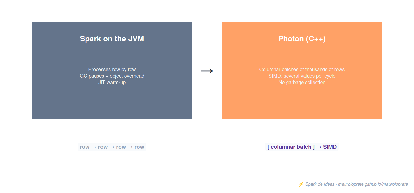
Spark executes queries on the JVM — the Java virtual machine, the environment where almost the entire big data ecosystem runs. That worked for a decade, but it carries three structural costs:
- Garbage collection (GC) pauses: the JVM periodically stops everything to clean up memory that’s no longer in use.
- The JIT (just-in-time compiler) warm-up: the JVM translates code into machine instructions while the program runs, so the first few minutes are always slower.
- The per-object memory overhead: every row drags along extra bytes of Java-specific internal structure.
None of this was a big deal when the bottleneck was disk. But with SSDs and columnar formats, the bottleneck moved to the CPU — and these three costs became the main problem.
Photon attacks exactly that: it replaces JVM execution with a native C++ runtime that processes data in columnar batches of thousands of rows, enabling SIMD instructions (Single Instruction, Multiple Data: the processor applies the same operation to several values at once, in a single cycle). Sequential memory access (column by column, not row by row) maximizes memory bandwidth and processor pipeline efficiency.
The key design point: Catalyst is still the optimizer. Photon doesn’t replace Spark’s planner, it replaces the execution layer. That’s why it’s compatible with Spark’s APIs — SQL and DataFrames in Python, R, Scala, and Java — with no code changes.
Note
According to the TPC-DS benchmarks (the industry standard for comparing analytical engines: a set of retail queries over synthetic data) published by Databricks, Photon delivers up to 5x better price/performance than other cloud data warehouses. Like every vendor benchmark, treat it as an upper bound — we’ll build our own further down.
2. Where it runs (and where you’re already using it without knowing)
Photon isn’t a product you buy separately: it’s built into Databricks compute. The difference is where it’s on by default and where it’s opt-in:
| Compute | Photon |
|---|---|
| SQL Warehouses (serverless, pro, classic) | Always on — it’s the default engine |
| Serverless compute (notebooks, jobs) | Always on |
| Lakeflow Declarative Pipelines serverless | Always on |
| All-purpose and jobs compute classic | On by default in the UI — the Use Photon Acceleration checkbox |
| Classic declarative pipelines | Configurable per pipeline |
If you use SQL Warehouses (we covered them in Tips #9), you’ve already been running Photon on every dashboard and ad hoc query.
Important
If you create clusters via API (Clusters API, Jobs API) or via DABs, Photon does NOT turn itself on: you have to set runtime_engine: PHOTON explicitly. It’s a classic: the dev cluster created through the UI flies, the production job deployed through CI/CD crawls, and nobody understands why.
In a Databricks Asset Bundle, the job cluster looks like this:
resources:
  jobs:
    etl_ventas:
      name: etl-ventas
      job_clusters:
        - job_cluster_key: main
          new_cluster:
            spark_version: "17.3.x-scala2.13"
            node_type_id: Standard_E8ds_v5
            num_workers: 4
            runtime_engine: PHOTON   # <- without this, it runs on the classic JVM
And in the Pipelines API, the flag is photon: true.
3. What it accelerates: covered operators and expressions
Photon doesn’t cover 100% of Spark. It covers the operators that dominate the execution time of a typical analytical workload:
| Category | Coverage |
|---|---|
| Scan | Parquet, Delta, CSV, JSON — with filter pushdown, dictionary pruning, and row-group skipping |
| Joins | Hash join (replaces sort-merge), nested-loop, null-aware anti join, spatial joins |
| Aggregations | Hash aggregate, including Min/Max/MinBy/MaxBy over nested types |
| Shuffle | Columnar shuffle redesigned for large-scale joins |
| Sort / Window | Sort, TopK, Limit, window functions |
| Writes | Delta, Iceberg, and Parquet: INSERT, UPDATE, DELETE, MERGE INTO, CTAS (CREATE TABLE AS SELECT) |
| Expressions | Comparison, arithmetic, conditionals (IF/CASE), strings, casts, dates/timestamps |
| Types | Numeric, string/binary, decimal, date/timestamp, struct, array, map, variant, geometry/geography |
Two details worth underlining:
Joins change strategy. Photon replaces sort-merge joins with high-performance hash joins. If you’ve been fighting giant sort-merge joins, this alone can justify the switch.
The shuffle is columnar too. It’s not just operator execution: the shuffle was redesigned to move columnar batches, which increases throughput on large joins.
Tip
The expression list is representative, not exhaustive, and it grows with every runtime. If a specific function matters to you, verify it with EXPLAIN (section 5) on your DBR version instead of trusting blog lists — including this one.
4. The transparent fallback: your query never fails because of Photon
What happens when the query uses something Photon doesn’t support? Nothing dramatic: Photon falls back to the Spark runtime for that portion of the execution and the query still produces the correct result.
This has an important practical consequence: a single query can run partly in Photon and partly on the JVM. The execution plan becomes mixed, and every Photon → JVM transition means converting columnar data to rows (and back), which has its own cost.
Warning
The fallback is silent. No error, no warning in the notebook — just a query slower than you expected. That’s why section 5 (monitoring) isn’t optional: if you don’t measure how much of your query runs in Photon, you don’t know whether you’re getting your money’s worth or overpaying.
The usual suspects that force a fallback:
- UDFs (User Defined Functions: functions you write yourself in Python or Scala to use inside a query) in the middle of the plan
- The RDD API or Dataset API (Scala’s typed lambdas)
- Stateful streaming operators
- Specific expressions not yet covered
5. How to measure how much Photon your query uses
Don’t guess: Databricks shows you exactly which part of the plan ran in Photon.
On SQL Warehouses and serverless — Query Profile. The Execution Details view shows the percentage of task time that ran in Photon. In the plan, Photon operators appear in purple and standard ones in gray. One number: if your query spends less than 80% of its time in Photon, something (almost always a UDF or a format) is forcing a fallback.
On classic clusters — Spark UI. In the SQL/DataFrame tab, the DAG (the flow diagram of the plan, step by step) paints Photon operators orange and Spark ones blue. Visual and immediate.
In code — EXPLAIN. Photon nodes show up with a prefix in the physical plan:
spark.sql("""
    SELECT categoria, SUM(monto) AS total
    FROM ventas
    WHERE fecha >= '2026-01-01'
    GROUP BY categoria
""").explain()

# == Physical Plan ==
# AdaptiveSparkPlan isFinalPlan=false
# +- PhotonResultStage
#    +- PhotonGroupingAgg(keys=[categoria], functions=[finalmerge_sum(...)])
#       +- PhotonShuffleExchangeSource
#          +- PhotonShuffleMapStage
#             +- PhotonGroupingAgg(keys=[categoria], functions=[partial_sum(...)])
#                +- PhotonScan parquet ventas (filters: fecha >= 2026-01-01)
If instead of PhotonScan you see FileScan, or a ColumnarToRow shows up in the middle of the plan, there’s your transition to the JVM.
6. How to read a Spark query plan (without crying)
The EXPLAIN from the previous section is useless if the plan looks like hieroglyphics to you. The good news: 90% of the interpretation boils down to three rules and knowing half a dozen nodes.
Rule 1 — read it bottom-up. The most indented node (the leaf) is the first step: almost always a scan. The node at the very top is the result. The plan is a tree where data flows from the leaves to the root.
Rule 2 — Exchange = shuffle = the expensive node. Every Exchange (or PhotonShuffleExchange) means moving data between workers over the network. Count how many there are: it’s the best predictor of query cost. A GROUP BY adds one; a join between large tables adds two.
Rule 3 — the plan you see may not be the one that runs. The first line usually says AdaptiveSparkPlan isFinalPlan=false: with AQE (Adaptive Query Execution), Spark re-optimizes at runtime using real statistics from each stage. You see the final plan in the Spark UI after execution, not in the EXPLAIN beforehand.
Let’s look at a typical join with its annotated plan:
spark.sql("""
    SELECT s.region, SUM(v.monto) AS total
    FROM ventas v
    JOIN sucursales s ON v.store_id = s.store_id
    GROUP BY s.region
""").explain()

# == Physical Plan ==                          (read bottom-up)
# AdaptiveSparkPlan isFinalPlan=false           <- 6. AQE may re-optimize
# +- PhotonGroupingAgg(keys=[region],
#       functions=[finalmerge_sum(...)])        <- 5. final agg post-shuffle
#    +- PhotonShuffleExchangeSource             <- 4. shuffle by region (expensive)
#       +- PhotonGroupingAgg(keys=[region],
#             functions=[partial_sum(...)])     <- 3. pre-aggregates on each worker
#          +- PhotonBroadcastHashJoin           <- 2. sucursales travels whole
#             :- PhotonScan parquet ventas
#             :     (filters: store_id IS NOT NULL,
#             :      requiredSchema: store_id, monto)   <- 1. reads only 2 columns
#             +- PhotonShuffleExchangeSource [broadcast]
#                +- PhotonScan parquet sucursales
What this plan is telling you:
| What you look at | What it tells you |
|---|---|
PhotonScan + requiredSchema |
Column pruning: it only reads the columns the query needs. If you see 40 columns for a single-column SUM, something’s off (the classic intermediate SELECT *). |
filters: / PushedFilters: in the scan |
The filters were pushed down to the scan: entire row groups get discarded without being read. If your WHERE doesn’t show up here, you’re filtering after reading everything. |
BroadcastHashJoin |
The small table travels whole to every worker — no shuffle of the big one. It’s the cheap join; Spark picks it when the small table is under the broadcast threshold. |
SortMergeJoin |
The classic “heavy” join: shuffle + sort on both sides. With Photon you’ll see PhotonShuffledHashJoin instead — a hash join without the sort. |
partial_sum → finalmerge_sum |
Two-phase aggregation: each worker pre-aggregates before the shuffle, so the bare minimum travels over the network. This is normal and it’s fine. |
ColumnarToRow / RowToColumnar |
The Photon ↔︎ JVM toll we discussed in section 4. One at the end of the plan is normal; several in the middle are a fallback eating your speedup. |
Tip
On runtimes with Photon, the EXPLAIN output ends with a Photon Explanation section that explicitly lists which operators don’t run in Photon and why (a UDF, an unsupported expression). It’s the fastest way to diagnose a fallback without opening the Spark UI.
Note
For long plans, df.explain("formatted") is much more readable than the default: it numbers the operators, shows the compact tree on top and each node’s detail below. And to see the final post-AQE plan with real metrics (rows per stage, spill, timings), the place is the SQL/DataFrame tab of the Spark UI — where Photon nodes also show up in orange.
7. Lab: benchmark with/without Photon
Enough theory. The experiment is simple: same cluster, same code, with and without the checkbox. We build a TPC-DS-style table (sales with dimensions) big enough for the CPU to be the bottleneck, and throw a query with join + aggregation + window at it.
Step 1 — generate data (~200M rows, about 6 GB in Delta):
from pyspark.sql import functions as F

(
    spark.range(200_000_000)
    .withColumn("store_id", (F.col("id") % 500).cast("int"))
    .withColumn("item_id", (F.col("id") % 100_000).cast("int"))
    .withColumn("fecha", F.date_add(F.lit("2025-01-01"), (F.col("id") % 540).cast("int")))
    .withColumn("cantidad", (F.col("id") % 10 + 1).cast("int"))
    .withColumn("precio", F.round(F.rand(seed=42) * 500, 2))
    .write.mode("overwrite")
    .saveAsTable("lab.photon_bench.store_sales")
)
Step 2 — the query (scan + filter + implicit join via aggregation + window, all Photon territory):
import time

query = """
    WITH ventas_diarias AS (
        SELECT store_id, fecha,
               SUM(cantidad * precio) AS revenue,
               COUNT(DISTINCT item_id)  AS items_distintos
        FROM lab.photon_bench.store_sales
        WHERE fecha >= '2025-06-01'
        GROUP BY store_id, fecha
    )
    SELECT store_id, fecha, revenue,
           AVG(revenue) OVER (
               PARTITION BY store_id ORDER BY fecha
               ROWS BETWEEN 6 PRECEDING AND CURRENT ROW
           ) AS revenue_7d
    FROM ventas_diarias
    ORDER BY store_id, fecha
"""

runs = []
for i in range(5):
    spark.sql("CLEAR CACHE")
    t0 = time.perf_counter()
    spark.sql(query).write.mode("overwrite").format("noop").save()
    runs.append(time.perf_counter() - t0)

print(f"wall-clock: median {sorted(runs)[2]:.1f}s | runs: {[f'{r:.1f}' for r in runs]}")
Step 3 — run it twice: once on a cluster with runtime_engine: PHOTON and once on an identical cluster with STANDARD. The full lab (a bundle with both jobs, ready for databricks bundle run) is in spark-de-ideas-labs.
Tip
The noop sink is the honest benchmark trick: it executes the entire plan (scan, shuffle, aggregation, window) without writing anywhere, so you measure pure compute with no output I/O noise. And CLEAR CACHE between runs keeps the disk cache from inflating the results of the repeats.
The real results
I ran it on Azure Databricks: two identical job clusters (driver + 1 worker Standard_D4s_v3, DBR 17.3 LTS), the only difference being the runtime_engine. Five runs per engine:
| Engine | Runs (s) | Median |
|---|---|---|
| STANDARD (JVM) | 26.3 · 11.0 · 11.4 · 10.4 · 10.9 | 11.0s |
| PHOTON | 15.5 · 6.8 · 6.7 · 6.5 · 6.2 | 6.7s |
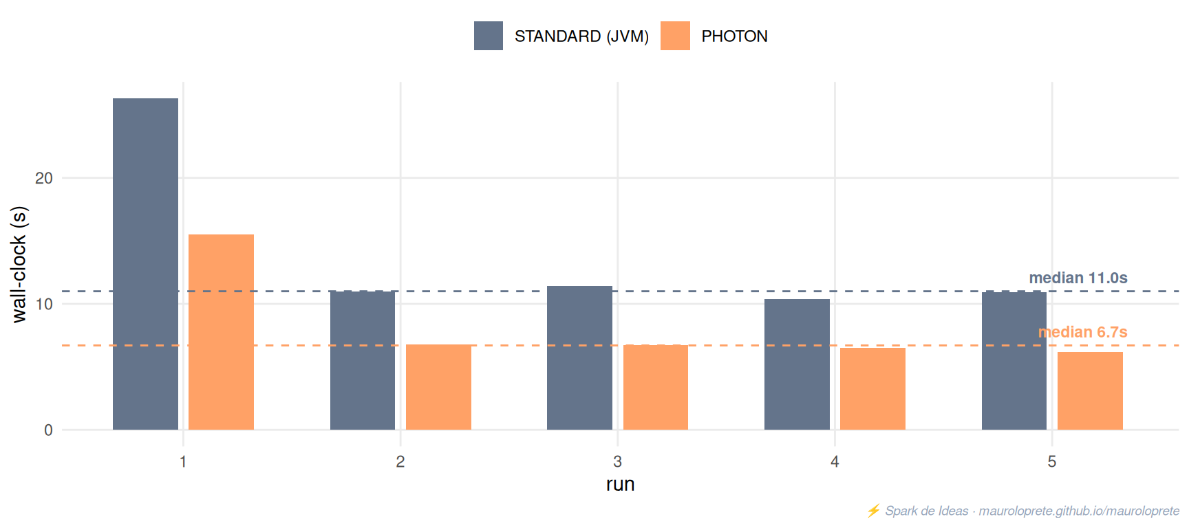
Speedup: 1.64x for this query, on this hardware. Three things to read from that:
- The first run lies on both engines (26.3s and 15.5s): it pays the JIT warm-up, the storage connections, and the shuffle initialization. That’s why the median and not the mean.
- 1.64x is less than the 2x-4x from the marketing benchmarks — and that’s how it should be: it’s a small cluster, a ~10-second query, and a 6 GB dataset. Photon’s speedup grows with scan size and aggregation complexity. This number is your floor, not your ceiling.
- Watch the DBU math (section 11): with a multiplier of ~2x, a 1.64x speedup on this workload doesn’t pay for itself in money — though it does in time. Exactly the kind of per-job decision we’re talking about.
And the execution plans the two runs returned — the same query, two worlds:
Sort [store_id ASC, fecha ASC]
+- Exchange rangepartitioning(store_id, fecha, 200)
   +- Window [avg(revenue) windowspecdefinition(...) AS revenue_7d]
      +- Sort [store_id ASC, fecha ASC]
         +- Exchange hashpartitioning(store_id, 200)
            +- HashAggregate(keys=[store_id, fecha], functions=[finalmerge_sum(...)])
               +- Exchange hashpartitioning(store_id, fecha, 200)
                  +- HashAggregate(keys=[store_id, fecha], functions=[partial_sum(...)])
                     +- Project [store_id, fecha, cantidad, precio]
+- Filter (fecha >= 2025-06-01)PhotonResultStage
+- PhotonColumnarToRow
+- PhotonSort [store_id ASC, fecha ASC]
+- PhotonShuffleExchangeSource
+- PhotonShuffleMapStage
+- PhotonShuffleExchangeSink rangepartitioning(store_id, fecha, 200)
+- PhotonWindow [avg(revenue) ... AS revenue_7d]
+- PhotonSort [store_id ASC, fecha ASC]
+- PhotonShuffleExchangeSource
+- PhotonShuffleMapStage
+- PhotonShuffleExchangeSink hashpartitioning(store_id, 200)
+- PhotonGroupingAgg(keys=[store_id, fecha], ...)Same tree, same steps — but in the second one even the shuffle is Photon (PhotonShuffleExchangeSink/Source), and the only ColumnarToRow sits at the end of the plan, where it belongs: a single conversion, right before returning the result.
The visual evidence: each run’s Spark UI
If you’ve never been in there: the Spark UI is the web console every Spark cluster ships with, showing the detail of what happened inside the engine. In Databricks you’ll find it on the cluster page (or the job run page), Spark UI tab. Inside there are tabs for Jobs, Stages, Executors… and the one we care about here: SQL/DataFrame, which lists every executed query with its duration, and clicking one shows you the DAG of the plan with real per-operator metrics — how many rows each node processed, how long each stage took. And in Databricks the nodes come color-coded: blue = JVM, orange = Photon. It’s literally seeing the fallback (or its absence) with your own eyes.
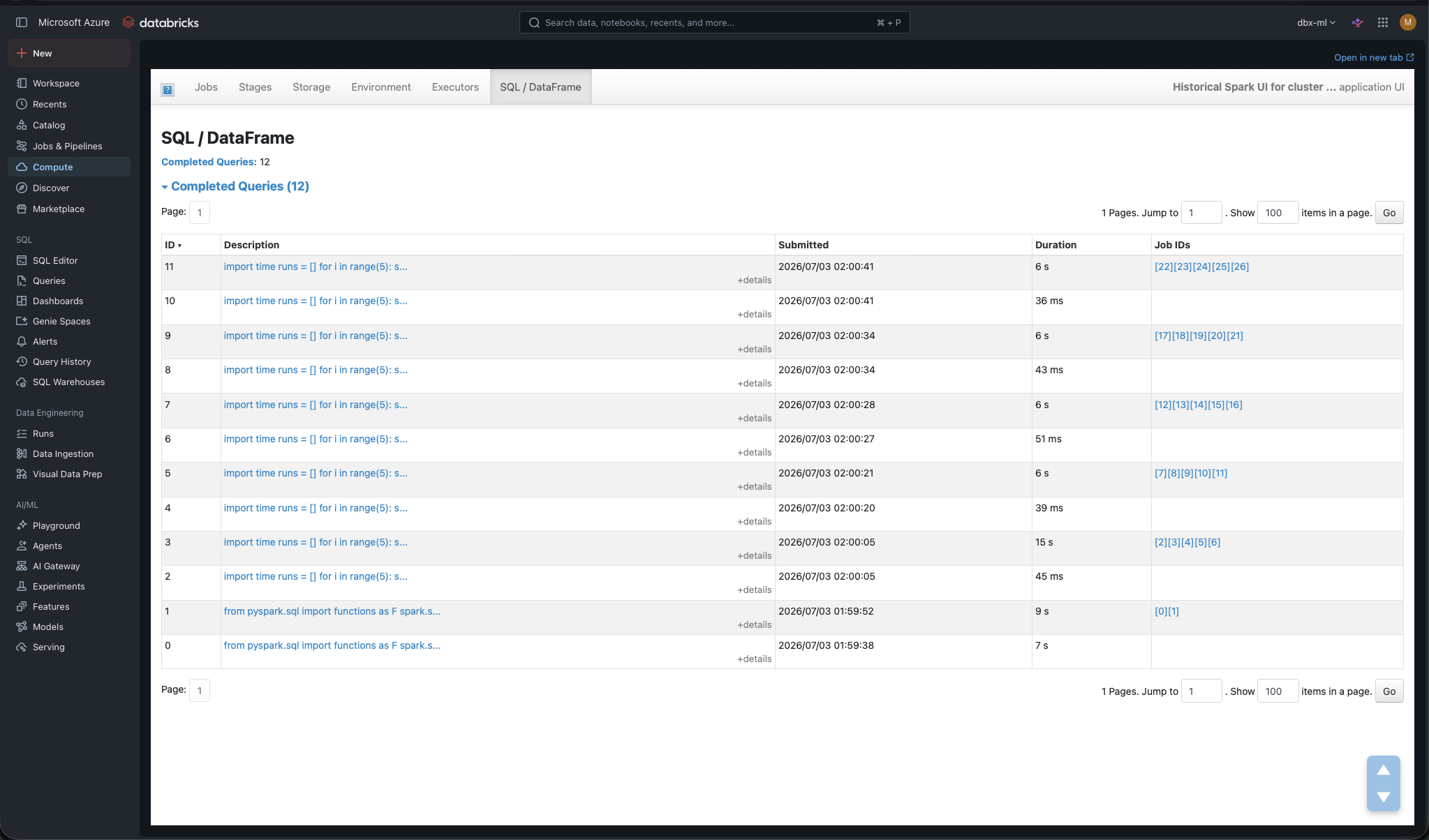
CLEAR CACHE, the count). Click any of them and the DAG opens with its metrics.This is what the two benchmark runs returned:
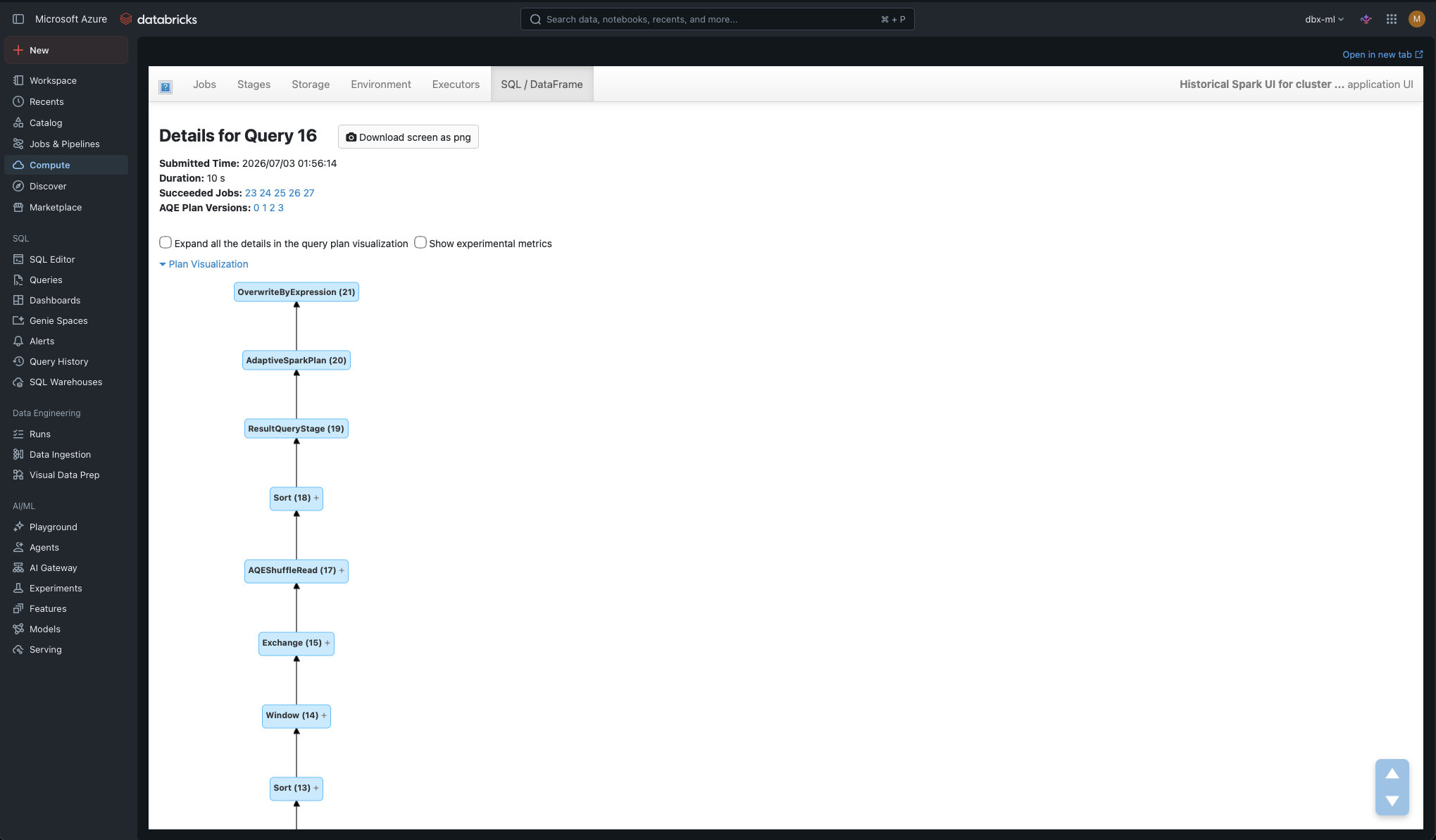
Exchanges, and the Window on top.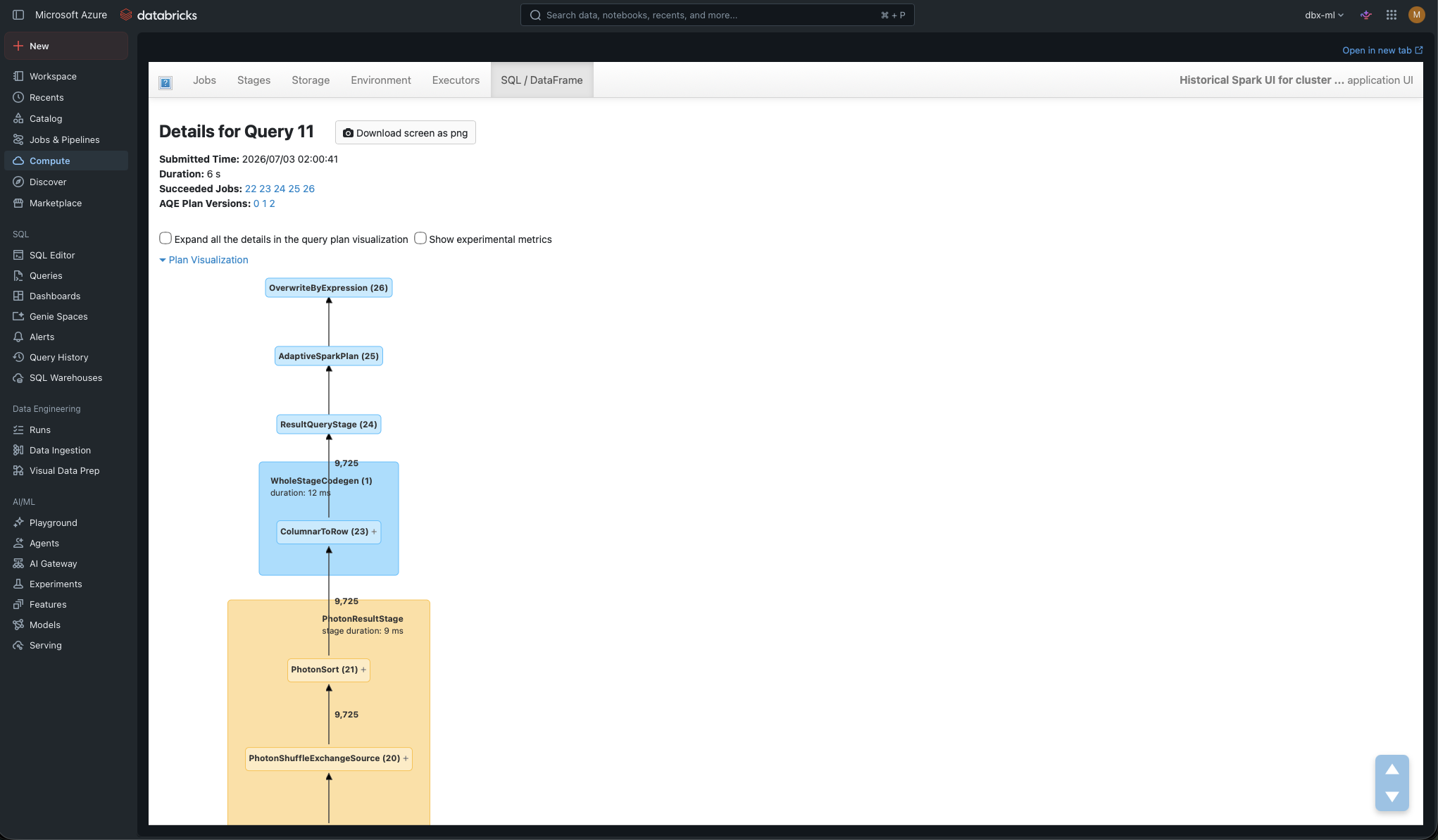
PhotonResultStage, PhotonSort, PhotonShuffleExchangeSource. The only blue block is the ColumnarToRow at the end — the single conversion to rows, where it belongs.And zooming into each plan’s detail, the per-operator numbers tell the whole story:
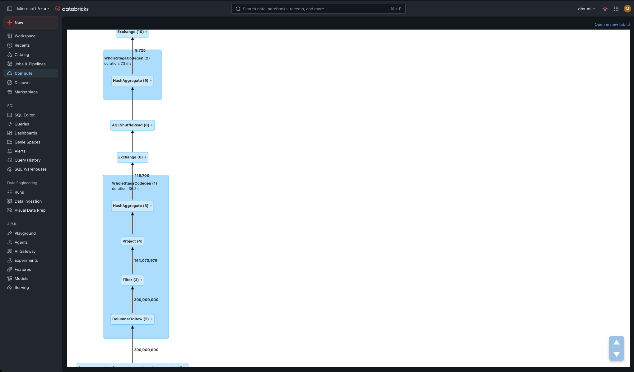
Filter receives 200,000,000 rows from the scan and lets 144,073,979 through: first it reads everything, then it filters. The WholeStageCodegen wrapping the HashAggregate racks up 36.2 s of task time — that’s the JVM generating code to process row by row.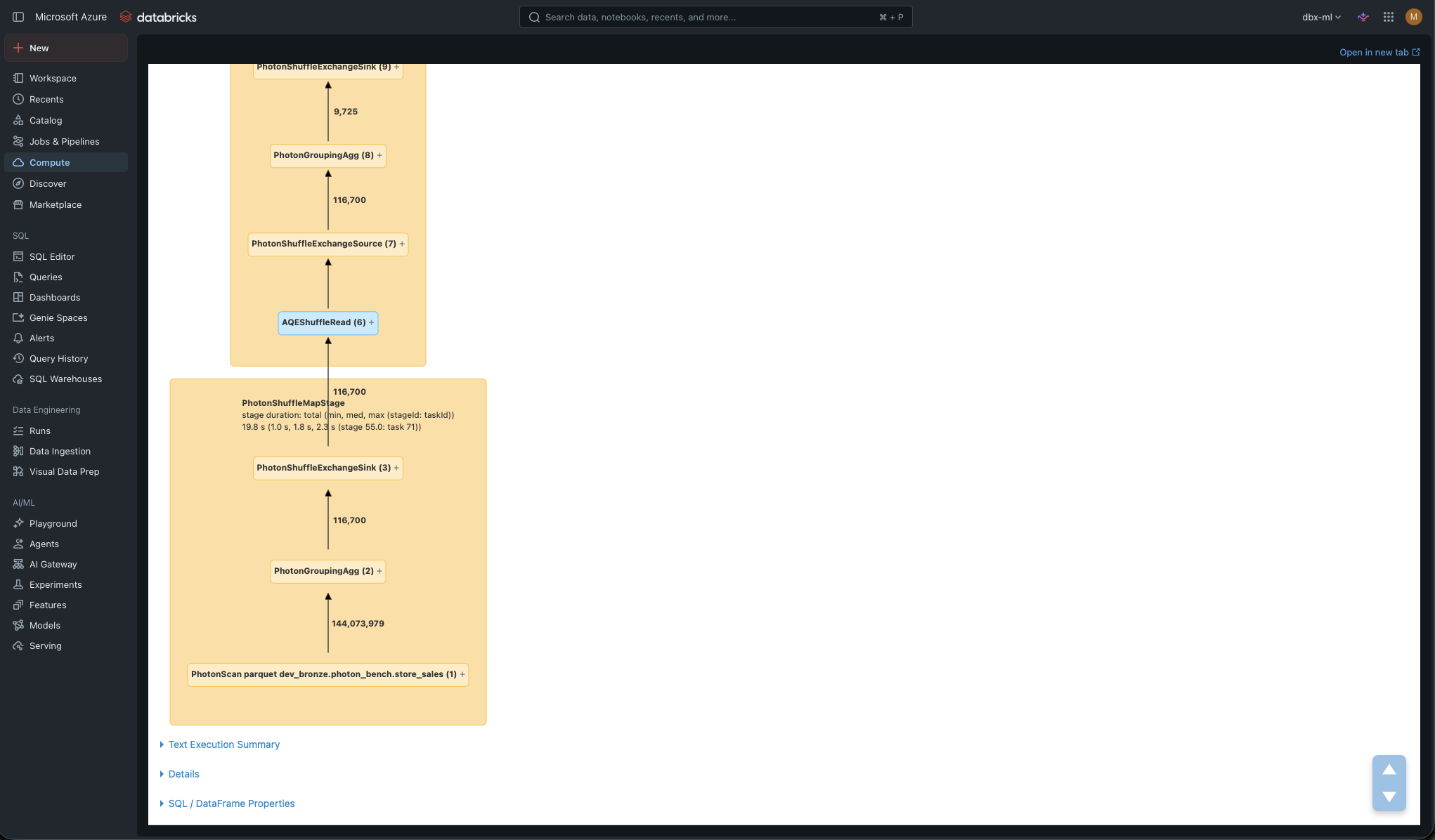
Filter node: the filter is embedded in the PhotonScan, which already delivers the 144,073,979 filtered rows. The PhotonGroupingAgg reduces them to 116,700 groups (500 stores × ~233 days) before the shuffle — the bare minimum travels over the network.Two facts hidden in those screenshots that are worth the zoom:
- The task time of the
WholeStageCodegen(36.2 s) on the JVM side is exactly the mechanism Photon replaces: Spark generates Java code at runtime for each query; Photon already is native code. - The 144M → 116,700 reduction before the shuffle is the
partial_sumfrom section 6 in action: it pre-aggregates on each worker and groups travel over the network, not rows.
Note
Lab bonus: in an earlier run, due to an Azure quota issue, the Photon cluster ended up with 1 worker against the STANDARD’s 2 — and it still won: 7.0s against 11.5s. Photon with half the hardware beat the JVM. Not the comparison I’d publish as a benchmark, but as an anecdote it says a lot.
While it runs, open the Spark UI and look at the DAG: on the Photon cluster the entire plan should be orange. If anything shows up blue, you’ve found a fallback — and an opportunity to understand why.
8. Writes: where Photon surprises
The reflex is to associate Photon with read queries, but the native Parquet writer also accelerates writes to Delta, Iceberg, and Parquet: INSERT, UPDATE, DELETE, MERGE INTO, and CREATE TABLE AS SELECT.
Two cases where this really shows:
- Wide tables: with hundreds or thousands of columns, the write improvement is especially significant. If you work with denormalized feature tables or legacy system extracts with 800 columns, this one’s for you.
- Heavy MERGEs: the MERGE in your CDC pipeline (Change Data Capture: replicating changes — inserts, updates, deletes — from a source system; we covered it with AUTO CDC in Tips #11) combines scan + join + write — the three things Photon accelerates at once.
9. The features that simply do NOT exist without Photon
Photon isn’t just “the same but faster”: there are platform optimizations that require Photon to be enabled:
- Predictive I/O for reads and writes — the heuristic that decides which files to read and how, key for deletion vectors and for speeding up point lookups.
- Dynamic file pruning in MERGE, UPDATE, and DELETE — without Photon, those DML operations don’t prune files dynamically and end up scanning far more than necessary.
Important
This is the argument usually missing from the cost discussion: turning Photon off on a job with big MERGEs doesn’t just take away the execution speedup — it turns off dynamic file pruning in the MERGE. The job doesn’t go back to “normal Spark speed”: it goes back to something worse than what you measured before optimizing.
10. What Photon doesn’t do (and won’t do for now)
The short but important list:
- UDFs: neither Python nor Scala. A UDF in the middle of the plan cuts off Photon execution and forces the jump to the JVM (columnar → rows conversion included). Before writing a UDF, exhaust the built-in functions — Photon’s expression coverage goes way beyond what people think.
- RDD API and Dataset API: if you have Scala code with typed lambdas (
ds.map(x => ...)), Photon doesn’t participate. The cost of the Dataset API’s “type safety” is now also measured in DBUs. - Stateful streaming: stateful aggregations,
mapGroupsWithState, stream-stream joins — not supported. Photon only accelerates stateless streaming (transformations + write to Delta/Parquet, with Delta, Parquet, CSV, JSON, Kafka, and Kinesis sources). - Queries under 2 seconds: the time goes to planning and scheduling, not execution. Photon can’t accelerate what doesn’t dominate the runtime.
11. The math: when the extra DBU pays for itself
First the acronym: the DBU (Databricks Unit) is the unit Databricks bills compute in — each instance type consumes a number of DBUs per hour, and you pay DBUs on top of the Azure VM cost. The detail that matters here: Photon instances consume DBUs at a higher rate than the same instances without Photon (the exact multiplier depends on the compute type — check it on the Azure Databricks pricing page).
The math is direct. If the job runs in time \(t\) at hourly cost \(c\), and with Photon it runs in \(t/s\) (speedup \(s\)) at hourly cost \(c \cdot m\) (multiplier \(m\)):
\[\text{Photon pays off if } s > m\]
With a typical multiplier close to 2x on jobs compute, you need a speedup greater than 2x to save money — plus you finish sooner, which also counts. CPU-bound workloads (where the bottleneck is the processor: wide aggregations, big joins, MERGEs, massive writes) usually clear it with room to spare; I/O-bound ones (dominated by reading or writing against disk and network, where the CPU is on vacation) or those full of UDFs, don’t.
Our lab from section 7 is the perfect example of the gray zone: a 1.64x speedup — the job finishes 40% sooner, but with a 2x multiplier the run comes out slightly more expensive. On a dataset 10x larger, that same query would probably cross the threshold. That’s why you do the math per job and with your own data, not with anybody else’s benchmark.
Tip
Don’t decide Photon “at the company level”: decide it per job. The section 7 benchmark takes 20 minutes to set up and gives you the real answer for your workload. Short, light, or UDF-heavy jobs → no Photon. Heavy SQL/DataFrame jobs → Photon, almost always.
12. Gotchas
- Clusters via API/DABs don’t enable Photon on their own. The UI ticks it by default, the API doesn’t:
runtime_engine: PHOTONor you’re running on the JVM without knowing. Audit your bundles today. - The fallback is silent. A new UDF in a pipeline that used to fly can double the runtime without anything failing. Metric to watch: % of task time in Photon in the query profile.
ColumnarToRowin the plan = a toll. Every Photon ↔︎ JVM transition converts formats. Many small transitions can eat the entire speedup.- Photon doesn’t fix the small files problem. The scan is more efficient even with small files, but you still pay listing and per-file overhead.
OPTIMIZEis still your friend. - Don’t expect anything on sub-2-second queries. If your dashboard fires 40 queries of 300ms, Photon isn’t your lever — look at the disk cache and the query design.
- The disk cache lies to you in benchmarks. The second run always looks better.
CLEAR CACHEor a fresh cluster between measurements. - Spot the engine: the plan tells you.
PhotonScanvsFileScanin theEXPLAINis the fastest smoke test to know whether you’re running where you think you’re running. - Streaming: check whether your pipeline is stateful before assuming a speedup. A
dropDuplicatesor a window aggregation in the stream makes it stateful — and there Photon doesn’t play.
13. When NOT to use Photon
| Situation | Why | Alternative |
|---|---|---|
| UDF-dominated jobs | Constant fallback, you pay the multiplier with no speedup | Refactor to built-ins first, Photon later |
| Short queries (<2s) | Planning dominates the time, not execution | Disk cache, serverless SQL warehouse |
| Stateful streaming | Not supported — everything runs on the JVM | Classic Structured Streaming (Tips #4) |
| RDD / Dataset API code | Photon doesn’t participate | Migrate to the DataFrame API (then Photon) |
| I/O-bound jobs (moving files, simple ingestion) | The bottleneck is network/storage, not CPU | Cheap compute without Photon |
| Zero migration budget and jobs already fast | No pain, no ROI to justify re-testing | Leave it for the next cycle |
References
Other posts in the series
If this post helped you, check out the previous Databricks Tips:
- Tips #1: Databricks Asset Bundles — IaC for Databricks
- Tips #2: Delta Lake — the 7 things you wish you’d known
- Tips #3: Unity Catalog — governance nobody implements well
- Tips #4: Structured Streaming — watermarks, triggers, and micro-batch
- Tips #5: MLflow + Unity Catalog — from experiment to model
- Tips #6: Feature Engineering — features that survive production
- Tips #7: Docker on Databricks — custom containers
- Tips #8: Jobs & Workflows — streaming and event-driven triggers
- Tips #9: SQL Warehouses — the compute that turns itself on
- Tips #10: AI Gateway — centralized governance for LLMs
- Tips #11: Lakeflow Declarative Pipelines — declarative pipelines with built-in quality
Next post in the series: Liquid Clustering, the replacement for partitions and Z-ORDER.